
Copy Files from SharePoint Online using Azure Data Factory and the Microsoft Graph API
In this post we’re discussing how to copy files from SharePoint Online using Azure Data Factory, the Microsoft Graph API and managed identity authentication.
Why use the Microsoft Graph API over the SharePoint API
A lot of existing documentation, including the official ADF documentation, references the SharePoint v1 API, but the v1 API is now considered legacy. The recommendation from Microsoft is that all SharePoint API calls use the SharePoint Online v2 API (Microsoft Graph API) instead.
The biggest benefit to this approach is that there is no need to obtain and pass around a bearer token. As a result, we can cut out the work of setting up service principals, managing those service principal credentials in Azure Key Vault and obtaining those service principal credentials at Azure Data Factory runtime.
Copy activities in both the SharePoint v1 and v2 APIs are executed using an HTTP connector. When using the SharePoint v1 API an Authorization header is required. The HTTP connector doesn’t support managed identity authentication. As a result, a bearer token must be obtained and used in the copy activity. In contrast, the Microsoft Graph API short-lived pre-authenticated download URLs (@microsoft.graph.downloadUrl) do not require an Authorization header to download a file. Therefore, we can use an anonymous HTTP connection to complete the download in the copy activity.
Web activities provide native support for user assigned managed identity, these can be used in both the SharePoint v1 and Graph API with managed identity authentication i.e. without a Authorization header and bearer token.
As a side note, The REST linked service does support managed identity authentication, but it does not support the necessary file based datasets that would be required for the file based copy activity.
Moving on to the task at hand…
For the purpose of this blog, we’re going to use a User Assigned Managed Identity. A System Assigned Managed Identity could also be used, with a few small changes to the instructions below,
The required steps are as follows
- Create a user assigned managed identity
- Grant Microsoft Graph API access rights to the user assigned managed identity
- Create Data Factory elements to navigate the Graph API and copy a file using the user assigned managed identity
Create a User Assigned Managed Identity
Programmatic access to the Graph API from Azure Data Factory is achieved using a user assigned managed identity. A user assigned managed identity can be created in the Azure Portal. Detailed steps below:
- Sign in to the Azure portal.
- Navigate to Managed Identities.
- Select Create
- Set appropriate values for Subscription, Resource Group, Location and Name in accordance with your environment
- Click on Review and Create
- Once created, note the Object (principal) ID in the resource Overview menu, you will need this later when assigning rights to the managed identity
Example:

Grant Graph API Access Rights to the User Assigned Managed Identity
It’s not possible to assign Graph API access rights to a user assigned managed identity in the Azure Portal. This must be done programatically. Based on requirements, the user assigned managed identity can be assigned the following rights.
| Permission | Description |
|---|---|
| Sites.Read.All | Read items in all site collections |
| Sites.ReadWrite.All | Read and write items in all site collections |
| Sites.Manage.All | Create, edit, and delete items and lists in all site collections |
| Sites.FullControl.All | Have full control of all site collections |
| Sites.Selected | Access selected site collections |
To copy files and navigate folders in this demo, we are going to assign the Sites.Read.All right. Best practice is to assign least privilege.
Using Powershell:
Connect-AzureAD
$ManagedIdentity = Get-AzureADServicePrincipal `
 -ObjectId "<Object (principal) ID>"
$GraphAPI = Get-AzureADServicePrincipal `
 -Filter "DisplayName eq 'Microsoft Graph'"
$SitesReadAll = $GraphAPI.AppRoles | where Value -like 'Sites.Read.All'
New-AzureADServiceAppRoleAssignment `
 -Id $SitesReadAll.Id `
 -ObjectId $ManagedIdentity.ObjectId `
 -PrincipalId $ManagedIdentity.ObjectId `
 -ResourceId $GraphAPI.ObjectId
Create Data Factory Elements to Navigate the Graph API and Copy a File
At this point we have a user assigned managed identity with read access to SharePoint Online via the Graph API. Consequently, we can now proceed to setup Azure Data Factory.
Register the User Assigned Managed Identity as a Credential in Azure Data Factory
- From within Azure Data Factory
- Navigate to Manage > Credentials
- Select New
- Name: Set appropriate value
- Type: User Assigned Managed Identity
- Azure Subscription: Select the subscription you used when creating the managed identity
- User Assigned Managed Identities: Select the managed identity you created
- Click on Create
Example:

Create Linked Services and Datasets to Support the Copy Activity
Below is a list of components we’ll need to create in Azure Data Factory for the copy activity.
- HTTP linked service for SharePoint Online
- Binary dataset that uses the HTTP linked service
- Azure Data Lake Gen2 linked service, this will be our sink for the purpose of this demo
- Binary dataset that uses the Azure Data Lake Gen2 linked service, this will be our sink dataset for the purpose of this demo
Create Linked Services
The sink components are not discussed in this post, additional detail and examples of Azure Data Lake Gen2 connectors can be found here.
Your HTTP linked service should use anonymous authentication and a parameter for passing in a dynamic URL. Configuration details below:
- HTTP linked service:
- Base URL: @{linkedService().URL}
- Authentication type: Anonymous
- Parameters: URL
Example:

Create Datasets
The sink components are not discussed in this post, additional detail and examples of Azure Data Lake Gen2 connectors can be found here.
- Binary Dataset
- Linked Service: Select HTTP linked service created above
- URL:
@dataset().URL - Parameter: URL, this will be used to pass the URL to the HTTP linked service
Example:

Create the Copy Activity Pipeline
We now have the necessary source and sink components in place to initiate a copy activity. Let’s put together a pipeline with a few activities that will ultimately download a file. In this pipeline demo we’re going to do the following:
- Get the SharePoint SiteID, subsequent API calls will require this
- Get a list of drives for the SharePoint site and filter this to the ‘Documents’ drive, this equates to https://<tenant>.sharepoint.com/sites/<site>/Shared%20Documents/ in my SharePoint tenant. Subsequent API calls require the Drive ID
- Get a download URL for a file in the Documents drive, pass this download URL onto a Copy activity
- Execute a copy activity that uses a HTTP source, referencing the download URL, and Data Lake Gen 2 sink
It’s well worth looking at the API documentation referenced below. There are multiple ways to navigate drives and search for files. Consequently, for your use case, you may find some methods more efficient than others.
Get the SharePoint SiteID
In a new empty pipeline create a web activity to fetch the SharePoint SiteID:
- Name: Get-SharePointSiteID
URL: https://graph.microsoft.com/v1.0/sites/<tenant>.sharepoint.com:/sites/<site> e.g. https://graph.microsoft.com/v1.0/sites/myTenant.sharepoint.com:/sites/mySite - Method: GET
- Authentication: User Assigned Managed Identity
- Resource: https://graph.microsoft.com
- Credentials: Select the credential you registered earlier
Store the SharePoint SiteID in a variable
Create a SiteURL variable, and use the output of the web activity above to set the variable to the SharePoint SiteID in a Set Variable activity
- Value:
@concat(
    'https://graph.microsoft.com/v1.0/sites/'
    ,activity('Get-SharePointSiteID').output.id
)
Get a list of drives for the SharePoint site
Create a web activity to fetch the list of drives:
- Name: Get-Drives
- URL:
@concat( variables('SiteURL') ,'/drives' ) - Method: GET
- Authentication: User Assigned Managed Identity
- Resource: https://graph.microsoft.com
- Credentials: Select the credential you registered earlier
Filter to the ‘Documents’ drive
Create a filter activity to filter to the Documents drive
- Name: Filter-Documents
- Items:
@activity('Get-Drives').output.value - Condition:
@equals(item().name,'Documents')
Get a download URL for a file in the Documents drive
Create a web activity to obtain a download URL for a file called data.csv in the General folder.
- Name: Get-File
- URL:
@concat( variables('SiteURL') ,'/drives/' ,activity('Filter-Documents').output.value[0].id ,'/root:/General/data.csv' ) - Method: GET
- Authentication: User Assigned Managed Identity
- Resource: https://graph.microsoft.com
- Credentials: Select the credential you registered earlier
Copy the file
Create a copy activity that uses a HTTP source, referencing the download URL
- Source dataset: Select the binary dataset you created earlier
- URL:
@activity('Get-File').output['@microsoft.graph.downloadUrl'] - Request Method: GET
Configure the sink based on your requirements. If you are using a binary source dataset (as per this demo) you will have to use a binary sink dataset.
Well, that about sums up how we copy files from SharePoint Online using Azure Data Factory and the Microsoft Graph API. I hope this helps you in your quest to remove those nasty bearer tokens from your workflows and move towards a world of managed identity.
Reference documentation
Partition Elimination with Power BI – Part 3, Integers
In part 1 and part 2 of this series we looked at how the SQL generated by Power BI in combination with the data type of the partition key in the source data can impact the likelihood of partition elimination taking place. We also discussed how the SQL statements generated by M & DAX convert date/datetime data types:
- DAX converts any flavour of date/datetime to a SQL datetime data type.
- Power Query converts any flavour of date/datetime to a SQL datetime2 data type.
| Partition Key Data Type | Date Filter Expression Language | Partition Elimination Possible | Expression Langauge Data Type Conversion |
|---|---|---|---|
| date | M | No | datetime2(7) |
| date | DAX | No | datetime |
| datetime | M | No | datetime2(7) |
| datetime | DAX | Yes | datetime |
| datetime2(7) | M | Yes | datetime2(7) |
| datetime2(7) | DAX | No | datetime |
| datetime2(other) | M | No | datetime2(7) |
| datetime2(other) | DAX | No | datetime |
| int | M | Yes | int |
| int | DAX | Yes | int |
Working with Integers
A fairly common way to implement dates/date partitioning on large fact tables in a data warehouse is to use integer fields for the partition key (e.g. 20191231). The good news is that both M and DAX will pass a predicate on the partition key through to SQL with no fundamental change to the data type i.e. partition elimination takes place as expected, joy!
The example below uses a simple measure against a DirectQuery data source, partitioned on an integer field.
Table Definition
create table dbo.MonthlyStuffInt (
  MonthDateKey int not null,
  TotalAmount decimal(10, 5) not null,
  index ccix_MonthlyStuffInt clustered columnstore)
on psMonthlyInt(MonthDateKey);
Power BI
In Power BI I have a slicer on the MonthDateKey column and a measure displayed in a card visual that sums TotalAmount.
Total Amount = SUM ( MonthlyStuff[TotalAmount] )

SQL Generated by Power BI
Using DAX Studio or Azure Data Studio to trace the above, I can capture the following SQL generated by the DAX expression:
SELECT SUM([t0].[Amount])
 AS [a0]
FROM
(
(select [_].[MonthDateKey] as [MonthDateKey],
    [_].[TotalAmount] as [Amount]
from [dbo].[MonthlyStuffInt] as [_])
)
 AS [t0]
WHERE
(
[t0].[MonthDateKey] = 20160501
)
Execution Plan
If I execute the query in SSMS, I can see that partition elimination takes place.

That all looks good, right?
It does indeed but we’d generally use a date dimension table to improve the browsability of the data model and when doing so, we could lose the partition elimination functionality we see above.
In the below example I have set up a date dimension table, related to a fact table, both using DirectQuery as the storage mode. To improve the browsability of the data model I’ve used the MonthYear field from the date dimension in the slicer, something I suspect is much more representative of the real world.
Table Definition
create table
   dbo.DimDate (
    DateKey int not null primary key clustered
    ,Date date not null
    ,MonthYear nchar(8) not null
  )
Power BI
Relationships

Visuals

SQL Generated by Power BI
SELECT SUM([t0].[Amount])
 AS [a0]
FROM
((select [_].[MonthDateKey] as [MonthDateKey],
    [_].[TotalAmount] as [Amount]
from [dbo].[MonthlyStuffInt] as [_]) AS [t0]

 inner join

(select [$Table].[DateKey] as [DateKey],
    [$Table].[Date] as [Date],
    [$Table].[MonthYear] as [MonthYear]
from [dbo].[DimDate] as [$Table]) AS [t1] on
(
[t0].[MonthDateKey] = [t1].[DateKey]
)
)

WHERE
(
[t1].[MonthYear] = N'Jun-2016'
)
Unfortunately, the generated SQL statement does not use partition elimination when querying the large fact table.
Workaround
One way to invoke partition elimination and improve the query performance of the underlying SQL is to introduce a cross-island relationship between the dimension table and the fact table in Power BI.

Put simply, by introducing the cross-island relationship Power BI will bypass the join to the Date dimension table in the underlying SQL and instead, the value/s of the relationship field (DimDate[DateKey]) will be passed directly to the fact table as part of the generated DirectQuery SQL.
SQL Generated by Power BI
SELECT SUM([t0].[Amount])
AS [a0]
FROM
(
(select [_].[MonthDateKey] as [MonthDateKey],
[_].[TotalAmount] as [Amount]
from [dbo].[MonthlyStuffInt] as [_])
)
AS [t0]
WHERE
(
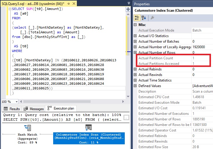
([t0].[MonthDateKey] IN (20160612,20160626,20160613
,20160627,20160614,20160601,20160615,20160628
,20160602,20160629,20160603,20160616,20160630
,20160617,20160604,20160618,20160605,20160619
,20160606,20160620,20160607,20160621,20160608
,20160609,20160622,20160623,20160610,20160624
,20160611,20160625))
)
A somewhat controversial recommendation as it’s in direct conflict with the Power BI documentation for filter propagation performance. My experience, especially in the context of large partitioned fact tables, is that the improvement you see in the data retrieval times from large fact tables (as a direct result of the ‘fact table only’ SQL statement and subsequent partition elimination) far outweighs any additional work required elsewhere.
To introduce this relationship type, change the storage mode of the date dimension table to Import.

Before:
Intra-Island Relationship (Date Dimension using DirectQuery, Fact using DirectQuery)

Profiled Query
SELECT SUM([t0].[Amount])
 AS [a0]
FROM
((select [_].[MonthDateKey] as [MonthDateKey],
    [_].[TotalAmount] as [Amount]
from [dbo].[MonthlyStuffInt] as [_]) AS [t0]

 inner join

(select [$Table].[DateKey] as [DateKey],
    [$Table].[Date] as [Date],
    [$Table].[MonthYear] as [MonthYear]
from [dbo].[DimDate] as [$Table]) AS [t1] on
(
[t0].[MonthDateKey] = [t1].[DateKey]
)
)

WHERE
(
[t1].[MonthYear] = N'Jun-2016'
)
Partition Elimination does not take place

After:
Cross-Island Relationship (Date Dimension using Import Storage Mode, Fact using DirectQuery)
Profiled Query
SELECT SUM([t0].[Amount])
 AS [a0]
FROM
(
(select [_].[MonthDateKey] as [MonthDateKey],
    [_].[TotalAmount] as [Amount]
from [dbo].[MonthlyStuffInt] as [_])
)
 AS [t0]
WHERE
(
([t0].[MonthDateKey] IN (20160612,20160626,20160613
,20160627,20160614,20160601,20160615,20160628
,20160602,20160629,20160603,20160616,20160630
,20160617,20160604,20160618,20160605,20160619
,20160606,20160620,20160607,20160621,20160608
,20160609,20160622,20160623,20160610,20160624
,20160611,20160625))
)
Partition Elimination takes place and we see a reduction in CPU and reads. The simplified query plan also came with the added benefit of aggregate pushdown on the columnstore index which would contribute to the improvement in performance.
Conclusion
If you are using a dimension table to improve the browsability of the data model, and you want to harness partition elimination to improve query performance in DirectQuery against very large fact tables then consider introducing a cross-island relationship between the dimension table and the fact table. This can be achieved by setting the dimension table to use Import mode. Familiarise yourself with the limitations before doing so and as always, profile your queries to ensure you’re obtaining optimal performance from your solution because one size never fits all.
Partition Elimination with Power BI – Part 2, Dates & DateTimes
In part 1 of this series we looked at how the SQL generated by Power BI, in combination with the data type of your partitioned columns in the source data, can impact the likelihood of partition elimination taking place. We also discussed how the SQL statements generated by M & DAX convert date/datetime data types:
- DAX converts any flavour of date/datetime to a SQL datetime data type.
- Power Query converts any flavour of date/datetime to a SQL datetime2 data type.
| Partition Key Data Type | Date Filter Expression Language | Partition Elimination Possible | Expression Langauge Data Type Conversion |
|---|---|---|---|
| date | M | No | datetime2(7) |
| date | DAX | No | datetime |
| datetime | M | No | datetime2(7) |
| datetime | DAX | Yes | datetime |
| datetime2(7) | M | Yes | datetime2(7) |
| datetime2(7) | DAX | No | datetime |
| datetime2(other) | M | No | datetime2(7) |
| datetime2(other) | DAX | No | datetime |
| int | M | Yes | int |
| int | DAX | Yes | int |
In this post, I’ll dig a little further into the detail and demonstrate the issue at hand with the use of some code snippets when working with a date column.
Setup
I have a SQL table shoved with some test data that I’ve partitioned by date (monthly) as follows:
create partition function pfMonthly (date)
as range right for values(
 '20190101','20190201'
,'20190301','20190401'
,'20190501','20190601'
);
create partition scheme psMonthly
 as partition pfMonthly all to ([PRIMARY]);
create table dbo.MonthlyStuff (
  MonthDateKey date not null
  , TotalAmount decimal(10, 5) not null
  , index ccix_MonthlyStuff clustered columnstore
) on psMonthly(MonthDateKey);
Power Query (M) –
Using the import storage mode, the following Power Query statement is used to filter a monthly slice of the data in Power BI.
let
    Source = Sql.Databases("mydbserver.database.windows.net"),
    mydb= Source{[Name="mydb"]}[Data],
    dbo_MonthlyStuff = mydb{[Schema="dbo",Item="MonthlyStuff"]}[Data],
    #"Filtered Rows" = Table.SelectRows(dbo_MonthlyStuff
      , each ([MonthDateKey] = #date(2019, 2, 1)))
in
    #"Filtered Rows"
Query folding takes place, producing the following native query (below). Note the correct data type (date) has been detected by Power Query however the native SQL query converts the filter to a datetime2:

Power Query Native Query – datetime2 Conversion
If I plug the generated SQL into SQL Server Management Studio and view the execution plan I can see that partition elimination does not take place against my partitioned table.
select
  [_].[MonthDateKey]
  , [_].[TotalAmount]
from
  [dbo].[MonthlyStuff] as [_]
where
  [_].[MonthDateKey] = convert(datetime2, '2019-02-01 00:00:00')

This is due to the misalignment of the data type in the predicate of the SQL statement (generated by M) with that of the data type of the partition key in the database. The source partition key is using the SQL date datatype and the SQL generated by M is casting the field to a datetime2.
To demonstrate this further, if I change the query manually in SSMS to use date conversion, partition elimination takes place resulting in much lower CPU and I/O overhead.
select
  [_].[MonthDateKey]
  , [_].[TotalAmount]
from
  [dbo].[MonthlyStuff] as [_]
where
  [_].[MonthDateKey] = convert(date, '2019-02-01 00:00:00')

Profiler Statistics without Partition Elimination
CPU: 4250000
Reads: 45684
Profiler Statistics with Partition Elimination
CPU: 578000
Reads: 4274
DAX
Now let’s demonstrate the issue using DAX with DirectQuery. If I use DirectQuery storage mode in Power BI and run a calculation against the underlying partitioned table, filtered to a particular month, I see a similar issue.
In Power BI I have a slicer on the MonthDateKey column (set as a date datatype) and a measure, that sums TotalAmount, displayed in a card visual.

Total Amount =
SUM ( MonthlyStuff[TotalAmount] )
The following SQL is generated by the DAX expression when using DAX Studio or Azure Data Studio to trace the above.
SELECT SUM([t0].[TotalAmount])
 AS [a0]
FROM
(
(select [$Table].[MonthDateKey] as [MonthDateKey],
    [$Table].[TotalAmount] as [TotalAmount]
from [dbo].[MonthlyStuff] as [$Table])
)
 AS [t0]
WHERE
(
[t0].[MonthDateKey] = CAST( '20190201 00:00:00' AS datetime)
)
As you can see from the below, once again we fail to harness the power of partition elimination. This is due to the misalignment of the data type in the predicate of the SQL statement (generated by DAX) and the data type of the source column. Partition elimination does not take place because the source column is using the SQL date datatype and the SQL generated by DAX is casting to a datetime data type.

To demonstrate this further, if I change the query manually in SSMS to use date conversion, partition elimination takes place and results in much lower CPU and I/O overhead.
SELECT SUM([t0].[TotalAmount])
 AS [a0]
FROM
(
(select [$Table].[MonthDateKey] as [MonthDateKey],
    [$Table].[TotalAmount] as [TotalAmount]
from [dbo].[MonthlyStuff] as [$Table])
)
 AS [t0]
WHERE
(
[t0].[MonthDateKey] = CAST( '20190201 00:00:00' AS date)
)

Profiler Statistics without Partition Elimination
CPU: 1640000
Reads: 27681
Profiler Statistics with Partition Elimination
CPU: 266000
Reads: 4274
Conclusion
If you want to harness partition elimination to improve query performance in DirectQuery mode and reduce load times in Import mode, then it’s worth keeping in mind how DAX and M convert the various date/datetime data types in the underlying SQL. As always, profile your queries and ensure they are performant before you commit.
In part 3 of this series we’ll look at partitioned tables that use an integer as the date partition key, a common practice in data warehousing.
Partition Elimination with Power BI – Part 1, Overview
This series will focus on the use of partition elimination when using Power BI to query partitioned tables in a Microsoft SQL Database (On-Prem or Azure).
Partition elimination can significantly improve Power BI DirectQuery performance. Similarly, Power BI Import models that target specific partition slices across very large datasets can see a reduction in load duration by using partition elimination. Unsurprisingly, as with all things tech, there are a few gotchas to look out for along the way. With partition elimination, the big gotcha is sensitivity to data type alignment between the predicate of the SQL query and the partition key of the partitioned table.
In this post, you’ll find an overview of the data type alignment issues we’re facing. Part 2 will cover some code examples and query plans to demonstrate the problem in more detail. My final write-up of the series will take a closer look at Power BI DirectQuery against tables partitioned on an integer datekey, a common practice in data warehousing.
Before we start, let’s briefly run through some terminology for those less familiar with table partitioning.
Table Partitioning
I won’t go into the details on this but in short, it’s a way of splitting large tables into smaller chunks which the SQL optimiser can (if it so chooses) access very quickly using a technique called partition elimination.
Check out the official Microsoft documentation for full details, and peruse this excellent post written by Cathrine Wilhemsen for a great introduction to the topic.
Partition Elimination
Copping out once again, I won’t be going into the details. In essence, if you write a query against your partitioned table which includes a filter on the partition key then partition elimination can take place, provided the optimiser deems it so :-). This detailed post by Kendra Little discusses the query performance we’re aiming to achieve via the dynamic SQL generated by Power BI.
What’s in a Data Type?
….well, everything. As powerful as partition elimination can be, it’s a sensitive beast. You need to make sure the data types used in your query align exactly with the data type of your partition key in your database. An example of this sensitivity is covered in this great post by Kendra Little.
No big deal, right? Provided you have control over the SQL syntax then it’s no big deal. However, with Power BI we’re at the mercy of the application and the SQL that Power BI generates via DAX & M.
DAX & M SQL Generation in Power BI
The SQL generated by a DAX expression against a DirectQuery datasource will cast dates and datetimes as a SQL datetime datatype e.g. cast('20190909' as datetime). The SQL generated by a M expression will cast dates and datetimes as a SQL datetime2 data type with default precision e.g. cast('20190909' as datetime2).
What’s the impact of this? Well, for example, if you’re running DirectQuery against large fact tables that are partitioned on a date data type and your Power BI Analysis includes a date filter on the partition key, partition elimination will not take place as the underlying dynamic SQL from Power BI will cast your date filter into a datetime or datetime2 data type, depending on the expression language used i.e. DAX or M.
The below table provides a summary of where partition elimination will and won’t take place.
| Partition Key Data Type | Date Filter Expression Language | Partition Elimination Possible | Expression Langauge Data Type Conversion |
|---|---|---|---|
| date | M | No | datetime2(7) |
| date | DAX | No | datetime |
| datetime | M | No | datetime2(7) |
| datetime | DAX | Yes | datetime |
| datetime2(7) | M | Yes | datetime2(7) |
| datetime2(7) | DAX | No | datetime |
| datetime2(other) | M | No | datetime2(7) |
| datetime2(other) | DAX | No | datetime |
| int | M | Yes | int |
| int | DAX | Yes | int |
Azure Data Factory Development with GitFlow – Part 1
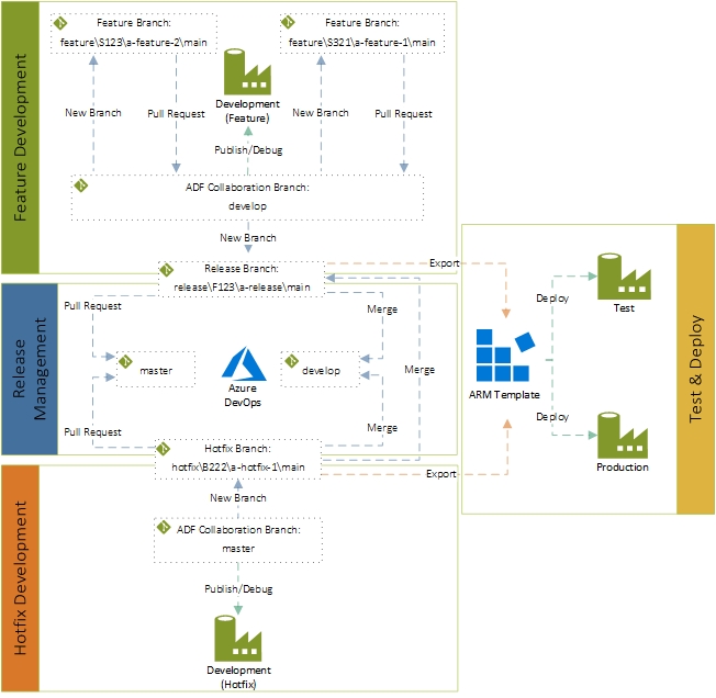
If you’re using or planning to use Git integration with Azure Data Factory then it’s well worth taking the time to define a suitable branching model for managing the various life-cycles of your project (think feature, hotfix and release). In this short series, I’ll discuss how we can structure our Azure Data Factory development with GitFlow, an easy to comprehend branching model for managing development and release processes.
Part 2: Implementation Detail
In part 1 of this series, you’ll get an overview of the various components which make up the solution. I’ll follow this up in part 2 with the implementation detail on how to deploy and configure your Data Factory environments to tie them in with the workflow. If all goes to plan we should land up with something along the lines of the below:
Component Overview
Now that we sort of know where we’re heading, let’s take a closer look at a few of the components that will make up the solution, namely:
- Git integration in Azure Data Factory UI for maintaining our source code
- GitFlow branching model, a structured approach to align our source code with the project life-cycle
- Continuous integration and delivery (CI/CD) in Azure Data Factory for the deployment of Data Factory entities (pipelines, datasets, linked services, triggers etc.) across multiple environments
- Azure DevOps for additional controls not available in the Azure Data Factory user interface
- Azure Data Factory for obvious reasons
Git integration in Azure Data Factory UI
With Azure Data Factory Git integration you can source control your Data Factory entities from within the Azure Data Factory UI, unfortunately, it does come with a few bugbears:
- Changes to the Data Factory automatically result in a commit e.g. new ADF entity (pipeline, connection etc.) = new commit
- Assigning Azure DevOps work items to a commit is not possible (use Azure DevOps instead)
- Merging between branches is only possible as part of a pull request
- The ability to publish a Data Factory is available from the collaboration branch only
For a more detailed look at the Git integration functionality in Azure Data Factory, have a read through the official documentation.
GitFlow branching model
First introduced by Vincent Driessen, GitFlow is a branching model for Git repositories which defines a method for managing the various project life-cycles. As with all things in life, there are lovers and haters but personally, I’m very fond of the approach. Having used it successfully on numerous projects I can vouch that, on more than one occasion, it has saved me from a merge scenario not too dissimilar to Swindon’s Magic Roundabout.
For those of you not familiar with GitFlow it’s well worth spending a few minutes reading through the details at nvie.com. In summary, and for the purpose of this post, it uses a number of branches to manage the development life-cycle namely master, develop, release, hotfix and feature. Each branch maintains clean, easy to interpret code which is representative of a phase within the project life-cycle.

Continuous integration and delivery (CI/CD) in Azure Data Factory
Continuous integration and delivery, in the context of Azure Data Factory, means shipping Data Factory pipelines from one environment to another (development -> test -> production) using Azure Resource Manager (ARM) templates.
ARM templates can be exported directly from the ADF UI alongside a configuration file containing all the Data Factory connection strings and parameters. These parameters and connection strings can be adjusted when importing the ARM template to the target environment. With Azure Pipelines in AzureDevOps, it is possible to automate this deployment process – that’s possibly a topic for a future post.
For a more detailed look at the CI/CD functionality in Azure Data Factory, have a read through the official documentation.
Azure DevOps
Azure DevOps is a SaaS development collaboration tool for doing source control, Agile project management, Kanban boards and various other development features which are far beyond the scope of this blog. For the purpose of this two-part post we’ll primarily be using Azure DevOps for managing areas where the ADF UI Git integration is lacking, for example, pull requests on non-collaboration destination branches and branch merges.
Azure Data Factory
To support the structured development of a Data Factory pipeline in accordance with a GitFlow branching model more than one Data Factory will be required:
- Feature and hotfix branch development will take place on separate data factories, each of which will be Git connected.
- Testing releases for production (both features and hotfixes) will be carried out on a third Data Factory, using ARM templates for Data Factory entity deployment without the need for Git integration.
- For production pipelines, we’ll use a fourth Data Factory. Again, as per release testing, using ARM templates for Data Factory entity deployment without the need for Git integration.
Of course, there are no hard or fast rules on the above. You can get away with using fewer deployments if you’re willing to chop and change the Git repository associated with the Data Factory. There is a charge for inactive pipelines but it’s fairly small and in my opinion not worth considering if additional deployments are going to make your life easier.
…to be continued
That covers everything we need, I hope you’ve got a good overview of the implementation and formed an opinion already on whether this is appropriate for your project. Thanks for reading. Come back soon for part 2!
Dynamically Flatten a Parent-Child Hierarchy using Power Query M
Introduction
For those of you familiar with recursive common table expressions in SQL, iterating through a parent-child hierarchy of data is a fairly straight forward process. There are several examples available which demonstrate how one could approach this problem in Power Query M. In this post, we’ll use recursion and dynamic field retrieval to loop through and dynamically flatten a parent-child hierarchy using Power Query M.
Show and Tell
Before we begin, let’s take a quick look at an example of the function being invoked in Power BI. This should hopefully give you some idea of where we’re heading with this.

Dynamically Flatten a Parent-Child Hierarchy using Power Query M
Sample Data
Let’s look at some sample data to get a feel for the type of data the function requires as input and the resultant dataset the function will output.
Input
| ParentNodeID | ParentNodeName | ChildNodeID | ChildNodeName |
|---|---|---|---|
| 100 | Stringer | 2 | Shamrock |
| 200 | Avon | 201 | Levy |
| 200 | Avon | 202 | Brianna |
| 200 | Avon | 203 | Wee-Bey |
| 2 | Shamrock | 3 | Slim Charles |
| 3 | Slim Charles | 51 | Bodie |
| 3 | Slim Charles | 52 | Poot |
| 3 | Slim Charles | 53 | Bernard |
| 51 | Bodie | 61 | Sterling |
| 51 | Bodie | 62 | Pudding |
| 52 | Poot | 61 | Sterling |
| 52 | Poot | 62 | Pudding |
Output
| ParentNodeID | ChildNodeID1 | ChildNodeID2 | ChildNodeID3 | ChildNodeID4 | ParentNodeName | ChildNodeName1 | ChildNodeName2 | ChildNodeName3 | ChildNodeName4 | HierarchyLevel | HierarchyPath | IsLeafLevel | HierarchyNodeID |
|---|---|---|---|---|---|---|---|---|---|---|---|---|---|
| 100 | Stringer | 1 | 100 | false | 100 | ||||||||
| 100 | 2 | Stringer | Shamrock | 2 | 100|2 | false | 2 | ||||||
| 100 | 2 | 3 | Stringer | Shamrock | Slim Charles | 3 | 100|2|3 | false | 3 | ||||
| 100 | 2 | 3 | 51 | Stringer | Shamrock | Slim Charles | Bodie | 4 | 100|2|3|51 | false | 51 | ||
| 100 | 2 | 3 | 51 | 61 | Stringer | Shamrock | Slim Charles | Bodie | Sterling | 5 | 100|2|3|51|61 | true | 61 |
| 100 | 2 | 3 | 51 | 62 | Stringer | Shamrock | Slim Charles | Bodie | Pudding | 5 | 100|2|3|51|62 | true | 62 |
| 100 | 2 | 3 | 52 | Stringer | Shamrock | Slim Charles | Poot | 4 | 100|2|3|52 | false | 52 | ||
| 100 | 2 | 3 | 52 | 61 | Stringer | Shamrock | Slim Charles | Poot | Sterling | 5 | 100|2|3|52|61 | true | 61 |
| 100 | 2 | 3 | 52 | 62 | Stringer | Shamrock | Slim Charles | Poot | Pudding | 5 | 100|2|3|52|62 | true | 62 |
| 100 | 2 | 3 | 53 | Stringer | Shamrock | Slim Charles | Bernard | 4 | 100|2|3|53 | true | 53 | ||
| 200 | Avon | 1 | 200 | false | 200 | ||||||||
| 200 | 202 | Avon | Brianna | 2 | 200|202 | true | 202 | ||||||
| 200 | 201 | Avon | Levy | 2 | 200|201 | true | 201 | ||||||
| 200 | 203 | Avon | Wee-Bey | 2 | 200|203 | true | 203 |
Power Query M Function
The fFlattenHiearchy function consists of an outer function and a recursive inner function.
The outer function will:
- Identify the top level parents
- Trigger the flattening
- Bolt on a few metadata columns
The inner function will:
- Self join onto the input hierarchy table to identify the next level of children within the hierarchy
- Filter out rows where the parent = child, to avoid infinite recursion
Flatten the hierarchy
The below code is used to build the basic hierarchy structure:
(
  hierarchyTable as table
  ,parentKeyColumnIdentifier as text
  ,parentNameColumnIdentifier as text
  ,childKeyColumnIdentifier as text
  ,childNameColumnIdentifier as text
) as table =>
  let
    #"Get Root Parents" = Table.Distinct(
      Table.SelectColumns(
        Table.NestedJoin(hierarchyTable
          ,parentKeyColumnIdentifier
          ,hierarchyTable
          ,childKeyColumnIdentifier
          ,"ROOT.PARENTS"
          ,JoinKind.LeftAnti
        )
        ,{
          parentKeyColumnIdentifier
          ,parentNameColumnIdentifier
        }
      )
    ),
    #"Generate Hierarchy" = fGetNextHierarchyLevel(
      #"Get Root Parents"
      ,parentKeyColumnIdentifier
      ,1
    ),
    fGetNextHierarchyLevel = (
      parentsTable as table
      ,nextParentKeyColumnIdentifier as text
      ,hierarchyLevel as number
    ) =>
      let
        vNextParentKey = childKeyColumnIdentifier & Text.From(hierarchyLevel),
        vNextParentName = childNameColumnIdentifier & Text.From(hierarchyLevel),
        #"Left Join - hierarchyTable (Get Children)" = Table.NestedJoin(parentsTable
          ,nextParentKeyColumnIdentifier
          ,hierarchyTable
          ,parentKeyColumnIdentifier
          ,"NODE.CHILDREN"
          ,JoinKind.LeftOuter
        ),
        #"Expand Column - NODE.CHILDREN" = Table.ExpandTableColumn(#"Left Join - hierarchyTable (Get Children)"
          ,"NODE.CHILDREN"
          ,{
              childKeyColumnIdentifier
              ,childNameColumnIdentifier
          },{
              vNextParentKey
              ,vNextParentName
          }
        ),
        #"Filter Rows - Parents with Children" = Table.SelectRows(#"Expand Column - NODE.CHILDREN"
          ,each Record.Field(_,vNextParentKey) <> null
              and Record.Field(_,vNextParentKey) <> Record.Field(_,nextParentKeyColumnIdentifier)
        ),
        #"Generate Next Hierarchy Level" = if Table.IsEmpty(#"Filter Rows - Parents with Children")
          then parentsTable
          else Table.Combine(
            {
              parentsTable
              ,@fGetNextHierarchyLevel(
                #"Filter Rows - Parents with Children"
                ,vNextParentKey
                ,hierarchyLevel + 1
              )
            }
        )
      in
        #"Generate Next Hierarchy Level"
  in
     #"Generate Hierarchy"
Add additional metadata
Additional metadata columns can be added to the hierarchy by using the code below. My original approach was to update these columns in each iteration of the hierarchy and although the code was slightly more digestible in comparison to the below, I did find it came at the expense of performance.
#"Add Column - HierarchyPath" = Table.AddColumn(#"Generate Hierarchy",
      "HierarchyPath"
      ,each Text.Combine(
        List.Transform(
          Record.FieldValues(
            Record.SelectFields(_,
              List.Select(Table.ColumnNames(#"Generate Hierarchy")
                ,each Text.StartsWith(_,childKeyColumnIdentifier)
                  or Text.StartsWith(_,parentKeyColumnIdentifier)
              )
            )
          )
          ,each Text.From(_)
        )
        ,"|"
      )
      ,type text
    ),
    #"Add Column - HierarchyNodeID" = Table.AddColumn(#"Add Column - HierarchyPath",
      "HierarchyNodeID"
      ,each List.Last(Text.Split([HierarchyPath],"|"))
      ,type text
    ),
    #"Add Column - HierarchyLevel" = Table.AddColumn(#"Add Column - HierarchyNodeID",
      "HierarchyLevel"
      ,each List.Count(Text.Split([HierarchyPath],"|"))
      ,Int64.Type
    ),
    #"Add Column - IsLeafLevel" = Table.AddColumn(#"Add Column - HierarchyLevel",
      "IsLeafLevel"
      ,each List.Contains(
          List.Transform(
            Table.Column(
              Table.NestedJoin(hierarchyTable
              ,childKeyColumnIdentifier
              ,hierarchyTable
              ,parentKeyColumnIdentifier
              ,"LEAFLEVEL.CHILDREN"
              ,JoinKind.LeftAnti
              )
              ,childKeyColumnIdentifier
            )
            ,each Text.From(_)
          )
        ,List.Last(Text.Split([HierarchyPath],"|"))
      )
      ,type logical
    )
The whole caboodle
Below you will find the full code for the function along with some documentation towards the end. You can plug the below code straight into a blank query in Power BI and reference it from your hierarchy query to flatten it.
let
  fFlattenHierarchy = (
    hierarchyTable as table
    ,parentKeyColumnIdentifier as text
    ,parentNameColumnIdentifier as text
    ,childKeyColumnIdentifier as text
    ,childNameColumnIdentifier as text
  ) as table =>
  let
    #"Get Root Parents" = Table.Distinct(
      Table.SelectColumns(
        Table.NestedJoin(hierarchyTable
          ,parentKeyColumnIdentifier
          ,hierarchyTable
          ,childKeyColumnIdentifier
          ,"ROOT.PARENTS"
          ,JoinKind.LeftAnti
        )
        ,{
          parentKeyColumnIdentifier
          ,parentNameColumnIdentifier
        }
      )
    ),
    #"Generate Hierarchy" = fGetNextHierarchyLevel(
      #"Get Root Parents"
      ,parentKeyColumnIdentifier
      ,1
    ),
    fGetNextHierarchyLevel = (
      parentsTable as table
      ,nextParentKeyColumnIdentifier as text
      ,hierarchyLevel as number
    ) =>
      let
        vNextParentKey = childKeyColumnIdentifier & Text.From(hierarchyLevel),
        vNextParentName = childNameColumnIdentifier & Text.From(hierarchyLevel),
        #"Left Join - hierarchyTable (Get Children)" = Table.NestedJoin(parentsTable
          ,nextParentKeyColumnIdentifier
          ,hierarchyTable
          ,parentKeyColumnIdentifier
          ,"NODE.CHILDREN"
          ,JoinKind.LeftOuter
        ),
        #"Expand Column - NODE.CHILDREN" = Table.ExpandTableColumn(#"Left Join - hierarchyTable (Get Children)"
          ,"NODE.CHILDREN"
          ,{
              childKeyColumnIdentifier
              ,childNameColumnIdentifier
          },{
              vNextParentKey
              ,vNextParentName
          }
        ),
        #"Filter Rows - Parents with Children" = Table.SelectRows(#"Expand Column - NODE.CHILDREN"
          ,each Record.Field(_,vNextParentKey) <> null
              and Record.Field(_,vNextParentKey) <> Record.Field(_,nextParentKeyColumnIdentifier)
        ),
        #"Generate Next Hierarchy Level" = if Table.IsEmpty(#"Filter Rows - Parents with Children")
          then parentsTable
          else Table.Combine(
            {
              parentsTable
              ,@fGetNextHierarchyLevel(
                #"Filter Rows - Parents with Children"
                ,vNextParentKey
                ,hierarchyLevel + 1
              )
            }
        )
      in
        #"Generate Next Hierarchy Level",
    #"Add Column - HierarchyPath" = Table.AddColumn(#"Generate Hierarchy",
      "HierarchyPath"
      ,each Text.Combine(
        List.Transform(
          Record.FieldValues(
            Record.SelectFields(_,
              List.Select(Table.ColumnNames(#"Generate Hierarchy")
                ,each Text.StartsWith(_,childKeyColumnIdentifier)
                  or Text.StartsWith(_,parentKeyColumnIdentifier)
              )
            )
          )
          ,each Text.From(_)
        )
        ,"|"
      )
      ,type text
    ),
    #"Add Column - HierarchyNodeID" = Table.AddColumn(#"Add Column - HierarchyPath",
      "HierarchyNodeID"
      ,each List.Last(Text.Split([HierarchyPath],"|"))
      ,type text
    ),
    #"Add Column - HierarchyLevel" = Table.AddColumn(#"Add Column - HierarchyNodeID",
      "HierarchyLevel"
      ,each List.Count(Text.Split([HierarchyPath],"|"))
      ,Int64.Type
    ),
    #"Add Column - IsLeafLevel" = Table.AddColumn(#"Add Column - HierarchyLevel",
      "IsLeafLevel"
      ,each List.Contains(
          List.Transform(
            Table.Column(
              Table.NestedJoin(hierarchyTable
              ,childKeyColumnIdentifier
              ,hierarchyTable
              ,parentKeyColumnIdentifier
              ,"LEAFLEVEL.CHILDREN"
              ,JoinKind.LeftAnti
              )
              ,childKeyColumnIdentifier
            )
            ,each Text.From(_)
          )
        ,List.Last(Text.Split([HierarchyPath],"|"))
      )
      ,type logical
    )
  in
    #"Add Column - IsLeafLevel",
  //Documentation
  fFlattenHierarchyType = type function (
    hierarchyTable as (type table meta [
      Documentation.FieldCaption = "Hierarchy"
      ,Documentation.LongDescription = "A table containing a parent-child hierarchy"
      ]
    )
    ,parentKeyColumnIdentifier as (type text meta [
      Documentation.FieldCaption = "Parent Key Column Identifier"
      ,Documentation.LongDescription = "The name of the column used to identify the key of the parent node in the hierarchy"
      ,Documentation.SampleValues = { "ParentID" }
      ]
    )
    ,parentNameColumnIdentifier as (type text meta [
      Documentation.FieldCaption = "Parent Name Column Identifier"
      ,Documentation.LongDescription = "The name of the column used to identify the name of the parent node in the hierarchy"
      ,Documentation.SampleValues = { "ParentName" }
      ]
    )
    ,childKeyColumnIdentifier as (type text meta [
      Documentation.FieldCaption = "Child Key Column Identifier"
      ,Documentation.LongDescription = "The name of the column used to identify the key of the child node in the hierarchy"
      ,Documentation.SampleValues = { "ChildID" }
      ]
    )
    ,childNameColumnIdentifier as (type text meta [
      Documentation.FieldCaption = "Child Name Column Identifier"
      ,Documentation.LongDescription = "The name of the column used to identify the name of the child node in the hierarchy"
      ,Documentation.SampleValues = { "ChildName" }
      ]
    )
  ) as list meta [
    Documentation.Name = "fFlattenHierarchy"
    ,Documentation.LongDescription = "Returns a flattened hierarchy table from a parent-child hierarchy table input."
      & "The number of columns returned is based on the depth of the hierarchy. Each child node will be prefixed"
      & "with the value specified for the childNameColumnIdentifier parameter"
    ,Documentation.Examples = {
      [
      Description = "Returns a flattened hierarchy table from a parent-child hierarchy table"
      ,Code = "fFlattenHierarchy(barksdaleOrganisation, ""ParentNodeID"", ""ParentNodeName"", ""ChildNodeID"", ""ChildNodeName"")"
      ,Result = "{100,2,3,51,62,""Stringer"",""Shamrock"",""Slim Charles"",""Bodie"",""Pudding"",5,""100|2|3|51|62"",TRUE,62}"
        & ",{100,2,3,51,""Stringer"",""Shamrock"",""Slim Charles"",""Bodie"",4,""100|2|3|51"",FALSE,51}"
      ]
    }
  ]
in
  Value.ReplaceType(fFlattenHierarchy, fFlattenHierarchyType)
Final Thoughts
It looks fairly verbose but in reality, it’s just 10 steps to flatten a hierarchy and bolt on the metadata columns, you could probably blame my code formatting for thinking otherwise. Anyone who is used to seeing common table expressions in SQL will hopefully find the logic defined in the function familiar.
In terms of performance, I’ve not pitted this against other methods nor done any performance testing but I’ve executed it against a ragged hierarchy with 11 levels spanning several thousand rows and it spat out results fairly instantaneously.
Alias Azure Analysis Services using Proxies in Azure Functions
Introduction
This post details how to alias Azure Analysis Services using proxies in Azure Functions. A cost-effective, flexible and codeless solution to manage link:// protocol redirects for Azure Analysis Services.
Let’s have a quick recap of the aliasing functionality in Azure Analysis Services before we dive into the implementation detail for this solution.
Connecting to Azure Analysis Services from Power BI Desktop, Excel and other client applications requires end users to specify the Analysis Services server name. For example, when connecting to a server called myanalysisservices, in the UK South region, you would use the address: asazure://uksouth.asazure.windows.net/myanalysisservices. As you can see, it’s a fairly unwieldy and hard to remember approach for connecting to the server from client tools.
An alternate approach is to use a shorter server alias, defined using the link:// protocol e.g. link://<myfriendlyname>. The endpoint defined by the shorter server alias simply returns the real Analysis Services server name in order to allow for connectivity from the client tools. A shorter server alias will (amongst other benefits):
- Provide end users with a friendly name for connecting to the Azure Analysis Services server
- Ease the migration of tabular models between servers by removing any impact on end users and removing the need for large amounts of manual updates to client tool content post migration e.g. changing the datasource in all Power BI reports and Excel connected workbooks
Any HTTPS endpoint that returns a valid Azure Analysis Services server name can provide the aliasing capability. The endpoint must support HTTPS over port 443 and the port must not be specified in the URI.
Additional information on aliasing Azure Analysis Services can be found in the following Microsoft documentation: https://docs.microsoft.com/en-us/azure/analysis-services/analysis-services-server-alias.
Implementation Overview
Components
Implement aliasing for Azure Analysis Services by deploying and configuring the following components:
- CNAME DNS record – Provides your end users with a friendly server name for Analysis Services
- Azure Function App with proxy capabilities – Passes the Analysis Services server name to the client tools
The CNAME destination will be configured to point to the Azure Function App. The Azure Function App will be configured with a proxy entry to serve up the connection information for the Azure Analysis Services server.

Alias multiple servers using one CNAME record by configuring the destination Azure Function App with multiple proxy entries. Each of these proxy entries must be configured with a different route template e.g. link://<myCNAME>/<myProxyEntryRouteTemplate>. Please see implementation detail below for additional information.

Implementation steps
Deploy Azure Analysis Services aliasing by following the steps below (covered in detail later in this post):
- Provision an Azure Function App
- Create a CNAME record for the Azure Function App
- Add the CNAME record to the Azure Function App
- Create proxy entries for each Azure Analysis Services server
Costs
1million executions per month and 400K GB-s worth of resource consumption are provided free as part of the Azure Functions Consumption Pricing Plan. Aliasing provided by the proxy service should fall well within the minimum execution time (100ms) and memory consumption (128MB) thresholds of this price plan. This should put you at < 125K GB-s of resource consumption over 1million executions. After this, charges are £0.15 per 1 million executions (assuming the minimum resource consumption of 100ms runtime @ 128MB memory consumption).
There are alternative pricing plans available, detailed information on Azure Functions pricing can be found here: https://azure.microsoft.com/en-gb/pricing/details/functions/
Implementation Detail
Provision an Azure Function App
- Login to https://portal.azure.com
- Click on Create a resource
- Search for and select Function App
- Click on Create
- Complete the necessary fields on the new Function App blade to create a new Azure Function App.
Take note of the app name for the Azure Function App as you’ll need to use this when creating the CNAME record.
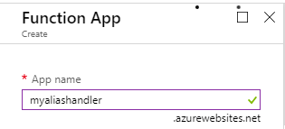
Please note that the name/URL of the Azure Function App is not the HTTPS endpoint which will be used as the alias by your end users. Feel free to name the Azure Funtion App in accordance with your naming conventions as the CNAME record will be used for friendly naming.
It is possible to configure delegated administration, for managing the Azure Function App proxy capability, by assigning the Website Contributor role on the Azure Function App access control list.
Create a new CNAME record for the Azure Function App
Create a new CNAME record with your domain service provider and set the destination for the record to the URL of the newly created Function e.g. myaliashandler.azurewebsites.net
Add the CNAME record to the Azure Function App
- Login to https://portal.azure.com
- Open the Azure Functions blade
- Load the blade for the newly created Azure Function App resource
- Click on Platform Features > Custom Domains

-
- Click on Add Hostname
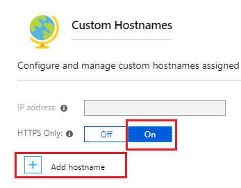
- Add the new hostname
- Click on Validate
- Once validated click on Add Hostname
- Add the SSL Binding by clicking on Add Binding next to the new hostname
- Select the relevant private certificate and click on Add Binding
Upload a private certificate to manage the SSL binding for the new hostname
- Load the blade for the newly created Azure Function App resource
- Click on Platform Features > SSL
- Choose the menu option, Private Certificate > Upload Certificate to upload your private certificate
- Load the blade for the newly created Azure Function App resource
- Click on Platform Features > Custom Domains
- Add the SSL Binding by clicking on Add Binding next to the new hostname
- Select the relevant private certificate and click on Add Binding
Create an alias entry for Azure Analysis Services on the Azure Function App
- Login to https://portal.azure.com
- Open the Functions App blade
- Click on the newly created Azure Function App resource
- Select the + symbol next to Proxies
Name: Add a meaningful name for the proxy
Route template: The path which will invoke this proxy entry
Allowed HTTP methods: GET
Set the following under Response Override
Status code: 200
Status message: accept
Under Headers:
Content-Type: text/plain
Body: The address to the Azure Analysis Services server e.g. asazure://<region>.asazure.windows.net/<server>

- On completion click create
You’ve now successfully configured an alias for your Azure Analysis Services server.
Testing
Azure Function App testing can be carried out in a web browser by connecting to: https://<myFunctionApp>/<myRouteTemplate> e.g. https://myaliashandler.azurewebsites.net/finance. The fully qualified Analysis Services server name should appear in the web browser.
Further testing can be conducted using the CNAME entry, in your web browser try connecting to https://<myCNAME.myDomain.com>/<myRouteTemplate> e.g. https://data.mydomain.com/finance
Finally, from within a client tool which supports the link protocol, connect using link://myCNAME.myDomain.com/<myRouteTemplate> e.g. link://data.mydomain.com/finance
Further Reading
https://docs.microsoft.com/en-us/azure/azure-functions/functions-proxies
https://docs.microsoft.com/en-us/azure/analysis-services/analysis-services-server-alias


